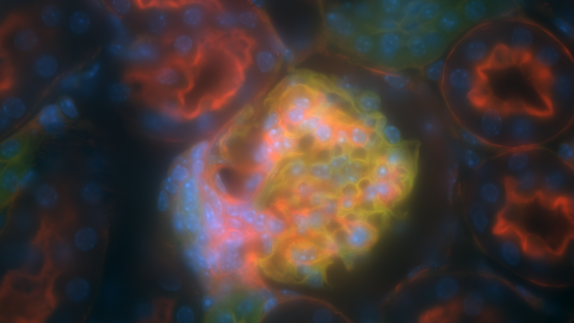
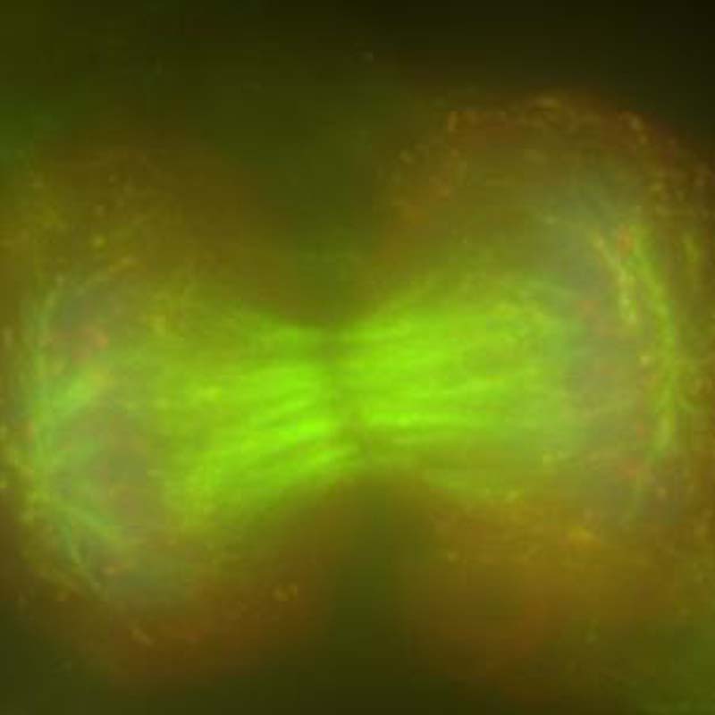
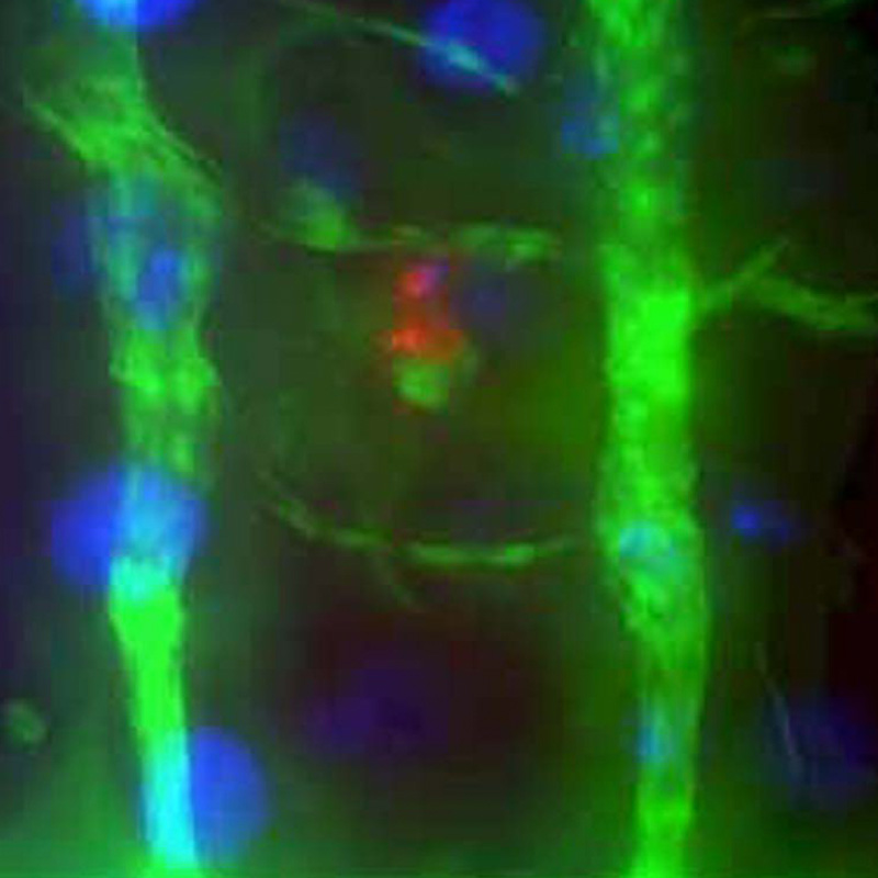
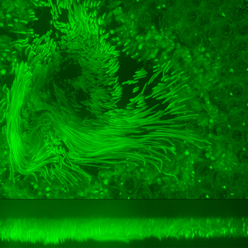
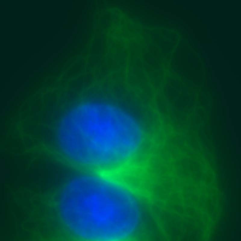
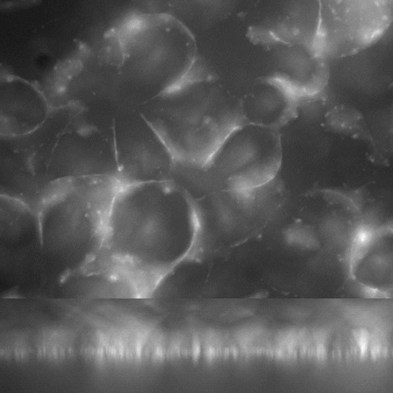
 After
After
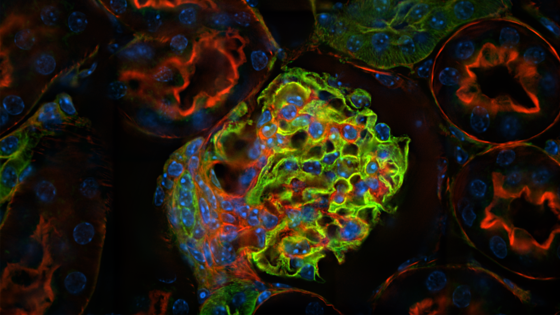
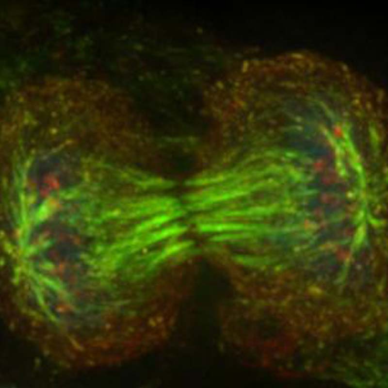
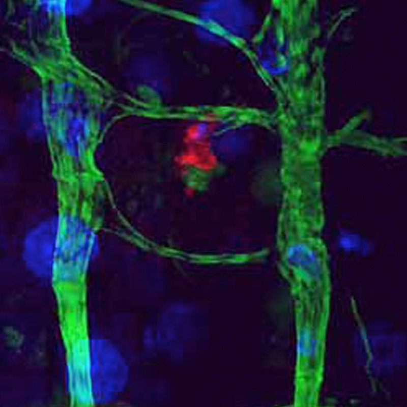
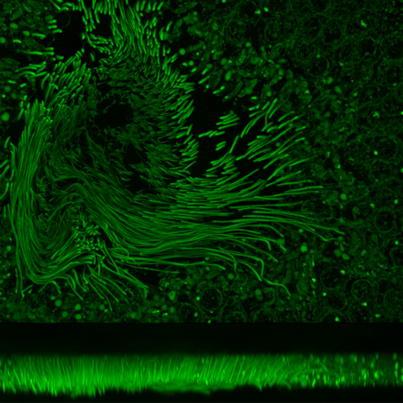
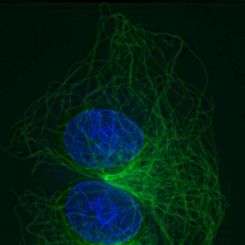
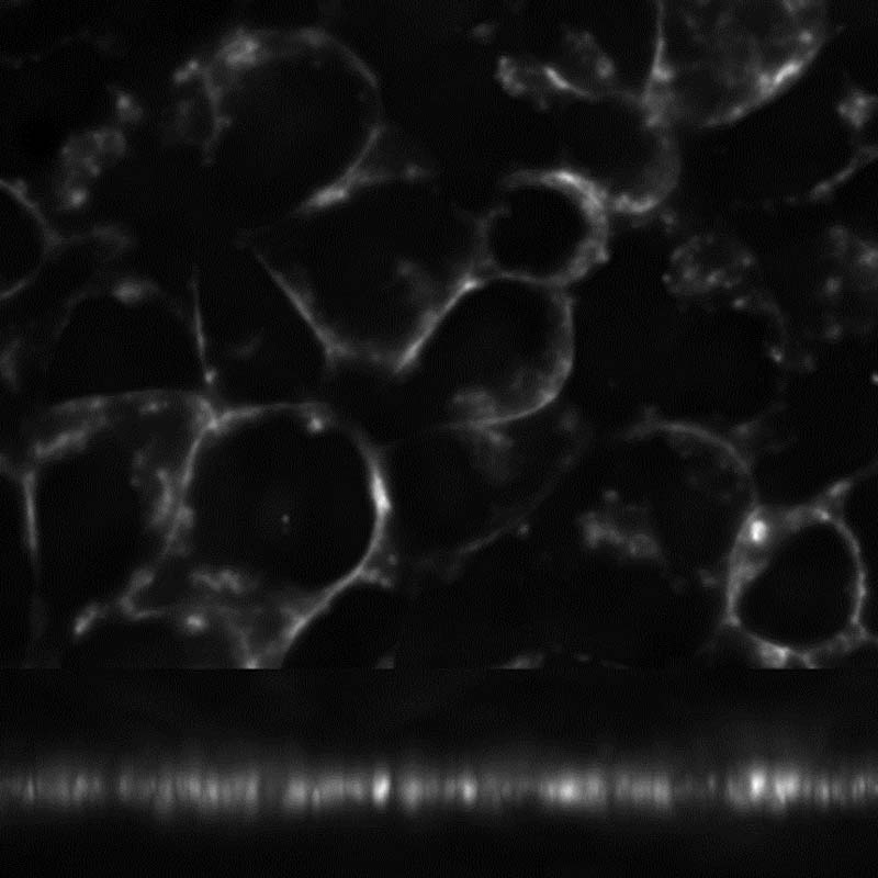
 Before
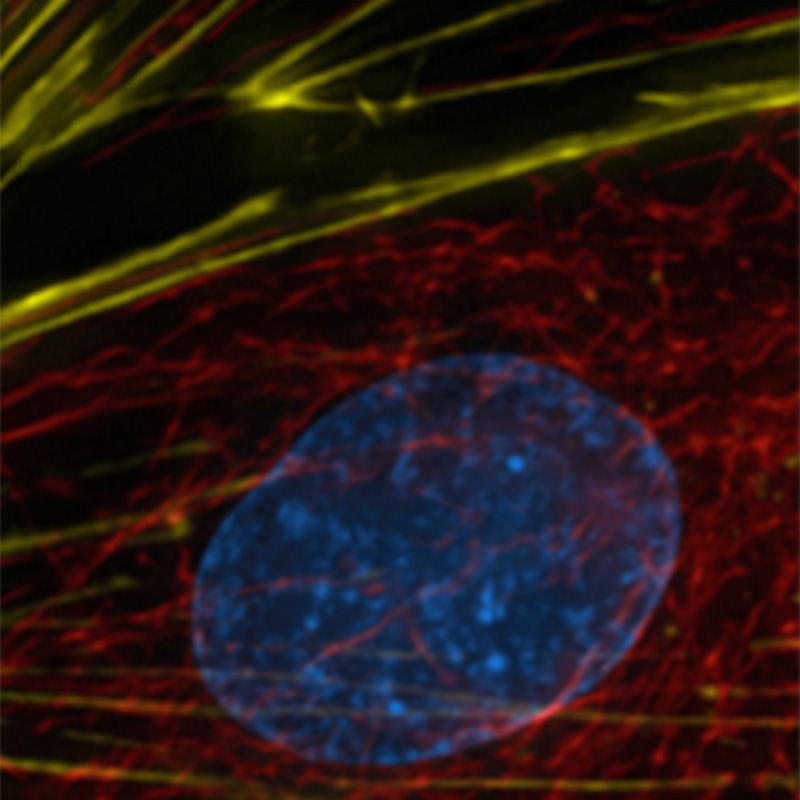
 After
After
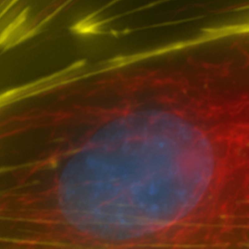
 Before
 After
After
 Before
 After
After
 Before
 After
After
 Before
 After
After
 Before
 After
After
 Before
 After
After
 Before
 After
After
 Before

AutoQuant
Image-Pro


| Standalone | New Module | |
|---|---|---|
|
Macro language |
|
|
|
OME file and metadata support |
|
|
|
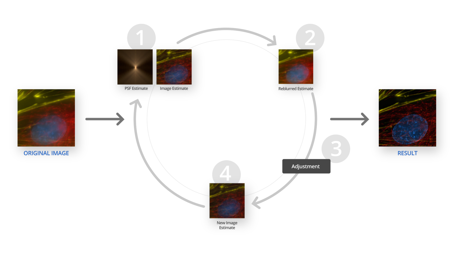
Theoretical PSF for STED Modality |
|
|
|
3D Movie Maker |
|
|
|
3D Viewer |
|
|
|
Image Adjustments and Correction |
|
|
|
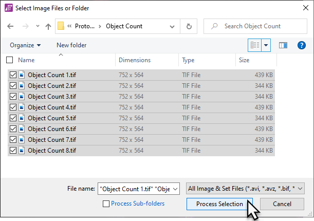
Image Import and Set Builder |
|
|
|
Spherical Aberration Correction |
|
|
|
Batch Processing |
|
|
|
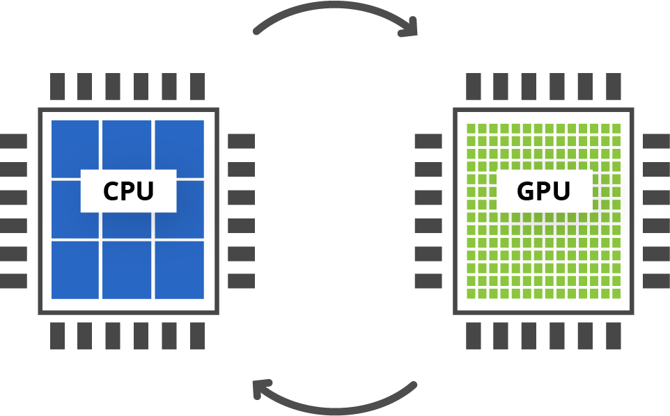
GPU Acceleration |
|
|
|
Inverse Filter |
|
|
|
No/Nearest Neighbors Algorithm |
|
|
|
DIC Restoration |
|
|